E-ISSN:2583-2468

Research Article

Stock Market

Applied Science and Engineering Journal for Advanced Research

2023 Volume 2 Number 2 March
Publisherwww.singhpublication.com

A Perceiving and Recognizing Automaton Prediction for Stock Market

Tere OP1*, Kshatriya D2
DOI:10.54741/asejar.2.2.4

1* Om Prakash Tere, Student, Department of Civil Engineering, Dr DY Patil College of Engineering, Pmpri, Pune, India.

2 Domesh Kshatriya, Guide, Department of Civil Engineering, Dr DY Patil College of Engineering, Pmpri, Pune, India.

The skill of forecasting the value of a company's equity on the stock market In order to forecast stock market prices, this research suggests a machine-learning (ML) artificial neural network model. The back-propogation algorithm is integrated into the suggested algorithm. Here, we use the back-propogation algorithm to train our ANN network model. Additionally, we conducted research using the TESLA dataset for this publication.

Keywords: back-propogation, artificial neural network, stock-market prediction

Corresponding Author How to Cite this Article To Browse
Om Prakash Tere, Student, Department of Civil Engineering, Dr DY Patil College of Engineering, Pmpri, Pune, India.
Email:
Tere OP, Kshatriya D, A Perceiving and Recognizing Automaton Prediction for Stock Market. Appl. Sci. Eng. J. Adv. Res.. 2023;2(2):19-25.
Available From
https://asejar.singhpublication.com/index.php/ojs/article/view/47

Manuscript Received Review Round 1 Review Round 2 Review Round 3 Accepted
2023-02-15 2023-03-01 2023-03-24
Conflict of Interest Funding Ethical Approval Plagiarism X-checker Note
None Nil Yes 12.95

© 2023by Tere OP, Kshatriya Dand Published by Singh Publication. This is an Open Access article licensed under a Creative Commons Attribution 4.0 International License https://creativecommons.org/licenses/by/4.0/ unported [CC BY 4.0].

Introduction

In past few decades, prediction of stock price is gaining more attention as profitability of investors in stock market is mainly depends on predictability. If direction of market is successfully predicted then investor can yield enough profit. For solving such kind of financial problem relationship between input and output is very complex so that’s why we have used ANN for solving or predicting stock price. An artificial neural network model is computer model whose architecture essentially mimics learning capability of human brain. The processing element of artificial neural network resembles biological structure of neuron and internal operation of human brain. In this paper , Multilayer feed forward back-propogation neural network is used for prediction purpose. Feed forward neural network is unidirectional connection between neurons that means information can flow only in forward direction. Here there is no connection between neurons present in same layer. Input has been fed into first layer and with help of hidden layers connected to last layer that produces output. And since all of information is constantly feeding forward from one layer to next hence it is called feed forward network. One of learning methods in multilayer Perceptron Neural Networks is error back-propogation in which network learns pattern in dataset and justifies weight of connections in inverse direction respect to gradient vector of error func. which usually regularized sum of Square error.

The back-propogation method picks a training vector from training data set and moves it from the input layer toward the output layer. In the output layer the error is calculated and propogated backward so the weight of the connection will be corrected.

This will usually go on until the error reaches a pre-defined value. Its proved that we can approximate any continuous function with a three layer feedback network with any precision.

It should be said that the learning speed will dramatically decreases according to the increase of the number of neurons and layer of the network.

Multilayer Feed Forward Perceptron

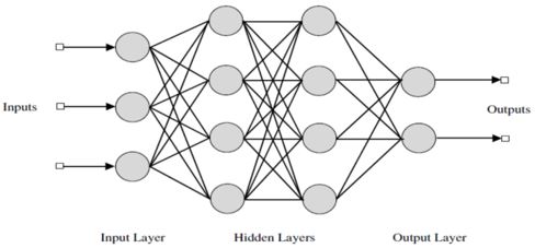
In this paper we have used multilayer feed forward perceptron below figure illustrate the how the multilayer feed forward perceptron looks like.

Multilayer: In multilayer neural network what happened there are more number of hidden layer are available in between the input layer and output layer called as hidden layer so in multilayer perceptron neural network more than one hidden layer are available.

Feed forward : in feed forward neural network what happened there is no edges are available in between the neurons present in the same layer here the synaptics are available in between only the neuron present in the different layer of neural network.


asejar_47_01.jpg
Figure 1:
Feed forward Multilayer Perceptron


Algorithms

Back-propogation Algorithm

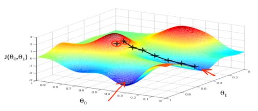
The back-propogation algorithm is falls into the general categ-ory of gradient descent algorithm. Purpose of gradient descent algorithm is to find the minima and maxima of a function by iteratively moving in the direction of negative slope of the function that we want to minimize or maximize.

asejar_47_02.jpg
Figure 2:
Gradient Descent

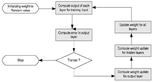
In back-propogation algorithm the network is trained by repete-dly processing the training data set and comparing the network output with the actual output if anything differs between the what output we are getting from our network and the desire output then this is called as error so after that what we are doing is we are again back propogate the whatever the output we got from our neural network to the back layer of the neural network till first hidden layer so that again our network will assign different weight randomly to the synaptic and try to generate the output with lesser error from the previous time and at every iteration our network output should be less from the output of previous time so that after some iteration we should get desire output and here we are keep back propogate the output from our neural network till our network trained completely. This below flowchart shows how back-propogation algorithm will work.

asejar_47_03.jpg
Figure 3:
Flowchart of Back-propagation Algorithm

Mathematical Derivation for Back-propogation Algorithm

In back-propogation our main intension is to find out the what changes is supposed to be happened on the weight assigned to the synaptic when the output we are getting from our network model is again backpropogated to the again first hidden layer so in this computation our main intension is to calculate ∆wij. First equation is about finding out the error generated from the neural network.

Ej (n) = dj (n) – yj (n) ..equ(1)

The above equation shows the error generated from our network and it can be calculated by just taking the difference of desired output and output we are getting from out neural network.


Here the term dj(n) will represent the desired output we are getting from out neural network and the term yj(n) is the output we got from our neural network . after that we found out the square error by just doing this.

E (n) = ½ ∑j€C ej2 (n) equ(2)

The above equation shows the error energy here we are actually intended to calculate the square energy by just doing square of all of the error and summing up the squared error we are getting from all of the neurons present in the output layer. Now we will find the average error energy.

Eavg (n) = 1/N ∑Nn=1 E(n) equ(3)

In above equation N is the number of iteration and we are summing up all the error energy from 1st iteration to N iteration for calculating the average error energy. Now we will calculate the value for induced field.

Vj(n) = ∑mi=1 Wij(n) * Yij(n) equ(4)

Local induced field value can be calculated by just doing summation of multiplication of Wij(n) and Yij(n) from number neurons in previous layer where is represent the number of neuron in previous layer and the value of Yij can be calculated by applying the activation function over induced field of Jth layer neuron below equation will illustrate this.

Yj(n) = ɸ(Vj(n)) equ(5)

Now we are intended to find out the what is change is happened in error with respect to change in the weight by just applying the chain rule of differentiation.

Here From equ(2) ej(n)

From equ(1) = -1

From equ(5)  = ɸ,(Vj(n))

From equ(4)  = Yj(n)

By putting this all of the value in equation 6 we got the following result:

-ej(n). ɸ,(Vj(n)). Yj(n) ..equ(7)

∆wij is applied to the Wij and which is proportional to the so according the definition of proportionality we can write as .

∆Wij = -η  equ(8)

In above equation η is constant of proportionality and the value of η is 9.25.from the equation (7) we can write equation (8) as .

∆Wij = η ej(n). ɸ,(Vj(n)). Yj(n)

δj(n) = ej(n). ɸ,(Vj(n)).  equ(9)

∆Wij = η δj(n) Yj(n)  equ(10)

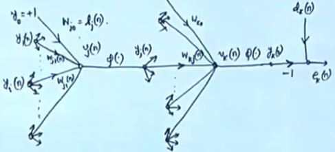
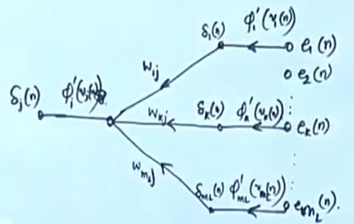
The below figure shows the signal flow of back-propogation algorithm .

asejar_47_04.jpg
Figure 4:
Signal Flow of Back-propagation Algorithm

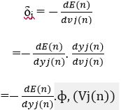
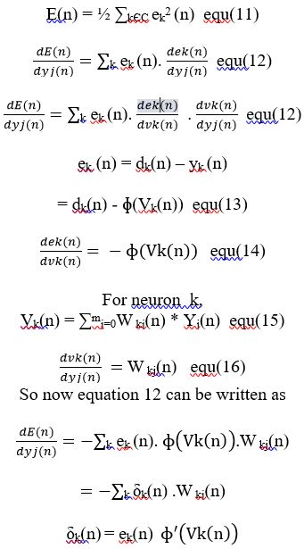
Now we can find out the δj,
asejar_47_05.jpg

Now as above figure if we consider k as output layer and j as preceding layer then calculation might looks likes:

asejar_47_06.jpg


So if we talk about back-propogation algorithm in a nutshell then It can be represented like this:

asejar_47_07.jpg
Figure 5:
Back-propagation Algorithm in Nutshell

Methodology

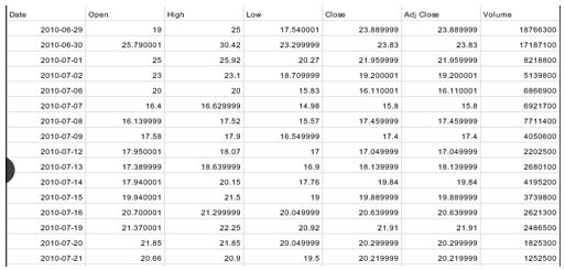
We will be using stock market data to predict closing price the workflow for the general neural network design has five primary steps:

a) Data collection and preparation

b) Network creation

c) Training the network

d) Validating the network

e) Using the network

asejar_47_08.jpg
Figure 6:
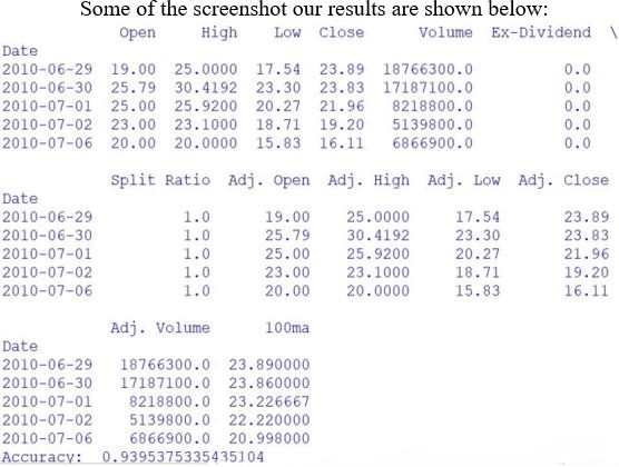
Tesla Data Set

a) Data Collection and Preparation

Data collection is the primary step and it is necessary in order to train, validate and test the neural network. For collection the data google finance has been used for collection the historical stock price details of any one of the company. This all of the data set are then feded into the network.

b) Network Creation

After collecting the all of the data set the next hectic task is to create your neural network model here the selection of what type of neural network is going to be difficult task. Neural network model like supervised or unsupervised and single layer or multilayer you should choose any one of those which is appropriate to solve your problem in our case it is supervise and multilayer perceptron.

c) Training the Network

As we are going to solve the problem with the help of artificial neural network then actually what we are trying to do is we are actually mimicking the functionality of biological neural to some extent since there is requirement of training your brain here also there is requirement of training your network for doing the task by itself once the your network trained this will perform every task correctly so for training the network there is lots of way but in our case we have used back-propogation algorithm because the efficiency of back-propogation algorithm is high very high as we are doing back propogate error.

d) Validating the Network

Once the training has done the network are validated using the validated data to enhance the performance of the network.


e) Using the Network

Once the network are optimized . It has been tested using the test data. In our case collected data of TESLA has been used to predict the adjusted closing price of stock.

asejar_47_09.jpg
Figure 7: Stock Data Set


asejar_47_10.jpg
Figure 8:
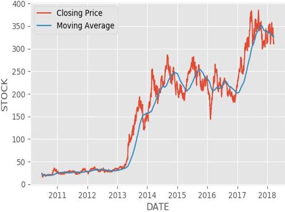
Closing and Moving Average


asejar_47_11.jpg
Figure 9:
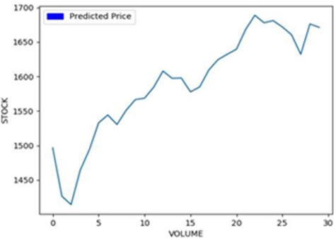
Predicted Price

Conclusion

By using historical stock market value information, we applied neural network models to forecast stock share values in these papers. Multilayer feed-forward networks are used to achieve this goal and address the issue. The outcome demonstrates that, with a 94% accuracy rate, there is no approach that is superior to the back-propogation algorithm for predicting the direction of changes in stock value.

References

1. Palavi Ranka. (2019). Stock market prediction using artificial neural networks. IME611 - Financial Engineering Indian Institute of Technology, Kanpur (208016), India.

2. Rosenblatt, F. (1997). The perceptron: A perceiving and recognizing automaton. Cornell Univ. NY. Project PARA Cornell Aeronaut Lab, pp. 85-460.

3. Mandic, D. P., & Chambers, J. A. (2001). Recurrent neural networks for prediction. John Wiley & Sons, LTD.

4. Goh, T. H., Wang, P. Z., & Lui, H. C. (1992). Learning algorithm for enhanced fuzzy perceptron. Proceedings of IJCNN, 2, pp. 435.

5. Lippmann, R.P. (1987). An introduction to computing with neural nets. IEEE Accost. Speech Signal Process. Mag., 4-22.